Pro-KMT gender gap? Think again!

Recently a foreign scholar asked me about the importance of gender in Taiwanese elections, and I gave the standard answer. Women are more likely to vote for the KMT than the DPP. This always surprises people unfamiliar with Taiwan. Do you mean that when a woman was one of the two main presidential candidates, more female voters supported the man?? Wait, I thought the DPP was a bit more progressive than the KMT. Are you saying that female voters preferred the more conservative party?? Well, yes.

However, I wondered whether that might be changing. More specifically, I wondered whether younger voters followed the same patterns as older voters. So I spent far too much time rummaging around in old survey data, and I came up with some interesting answers. The gender gap in 2020 was not like the previous three elections. And younger voters are, in fact, different.

In voting, the gender gap can be defined as the difference between support for two parties among men minus the difference among women [(A_m-B_m)-(A_f-B_f)]. This gives you a magnitude and a direction, so that we can say something like “women support Democrats 14 points more than Republicans, compared to men.”

I looked at the Taiwan Elections and Democratization Study (TEDS) post-election face-to-face surveys for each of the past five presidential elections. As you can see, there was a mild gap in 2004 in favor of the DPP. However, in 2008 and 2012 there were very big gaps in favor of the KMT. 2012 is the one that everyone paid attention to since Tsai Ing-wen was the first female presidential candidate representing a major party. However, this did not attract much support from women in the general electorate. The gender gap was much smaller in 2016, though it was still mildly in the KMT’s favor. In 2020, however, the gap had shifted in the other direction. In her third run, Tsai finally achieved a gender gap in her favor. It isn’t a huge gender gap, but it is markedly different from the previous three elections.

That’s the headline, but there is always more to dig up. After reflection, I decided to ignore 2004 in the rest of this post. There wasn’t much of a gender gap in 2004, and the jumbled data seemed to cause more confusion than clarity. At any rate, the patterns we have been talking about for the past decade emerge clearly with Ma Ying-jeou in 2008.

My suspicion is that younger voters are different from older voters. How should I define younger and older? Normally, we just break samples into ages 20-29, 30-29, and so on. That’s fine for a single survey. However, I’m looking at four-year intervals over a couple of decades. Nearly half of each group graduates to the next age group in each subsequent survey. Instead, I need to look age political generations, so that I’m looking at the same group of voters in each survey. There is a fairly large literature on political generations, and each scholar cuts the population slightly differently. Ideally, you would like each generation to go through the same critical formative experiences. I don’t want to get into those battles since I don’t have strong feelings about exactly where the lines between generations should be drawn. I’m simply going to borrow a definition from scholars who have thought extensively about this question. Lin Pei-ting, Cheng Su-feng, and T.Y. Wang recently published a paper on political generations and national identity, and since they are all knowledgeable and trustworthy scholars, I’ll just steal their definition.

cohort	Birth	Ages 2008	Size 2008	Ages 2020	Size 2020
5	1985-	23&under	7.2	35&under	26.7
4	1969-84	24-39	35.5	36-51	31.1
3	1954-68	40-54	31.1	52-66	25.7
2	1942-53	55-66	14.7	64-78	12.0
1	-1941	67&up	11.4	79&up	4.5

Cohort1, the oldest cohort, has been slowly aging out of the electorate. In 2008, there were still many C1 members who were active and energetic. Now, however, they are almost all octogenarians or older, and their share of the electorate[1] has declined to less than 5%.  At the other end of the spectrum, C5 were all still too young to vote in 2004, so they have slowly been aging into the electorate, making up a larger share in each election cycle. The middle three cohorts are largely the same people in each election. We probably won’t be able to say that much longer, since the oldest people in C2 are now nearing their 80^th birthdays. C3 and C4 represent Taiwan’s era of rapid population growth, and these are the largest two cohorts for most of the era we are looking at. In 2008, they accounted for roughly 2/3 of the electorate, and in 2020, they still made up 57%.

Rather than putting up one chaotic chart with too many jumbled lines to see a clear pattern, I’ll tell this story cohort by cohort. I start with the chart of all voters. Blue lines represent support for KMT and PFP presidential candidates, while green lines represent the DPP. Darker blue and green represent men and lighter blue and green represent women. You can see the national gender gaps quite clearly in this picture. In 2008, there is a huge gap between the light blue and light green lines, reflecting a 25% difference in support for Ma and Hsieh. The gap is about half that size among men. Hence, we get a double-digit gender gap in favor of the KMT in 2008. In 2012 and 2016, the two green lines are very close; there wasn’t much difference in support for the DPP among women and men. However, there is still a sizeable gap between the two blue lines; women gave significantly more support to the KMT than men did.[2] That gap disappeared in 2020, and a gap emerged between the two green lines.[3]  

C1, the oldest cohort, doesn’t show much of a gender gap in 2008 and 2012. The lines go in all crazy directions in 2016 and 2020, but we probably should ignore that. As a general rule of thumb, you shouldn’t pay attention to subgroups with fewer than 200 cases. In 2016 and 2020, C1 had shrunk so much that it was under 100 cases in the TEDS surveys. This isn’t the group creating the gender gap.

C2 does show a consistent pattern. For the blue side, there isn’t much difference between men and women. However, on the green side, women consistently give less support to the DPP than men.

C3 also shows a consistent pattern, though it is different from the C2 pattern. From one angle, it is the mirror image. In the first three elections, there wasn’t much difference on the green side, but women were consistently more supportive of the KMT than men. However, while C2 showed the same pattern all the way through 2020, C3 did not. In 2020, C3 suddenly reversed its previous pattern, with women swinging dramatically toward the DPP and away from the KMT.

C4 is very similar to C3. In the first three elections, there is a strong pro-KMT gender gap. However, in 2020 this suddenly reverses. Recall that C3 and C4 make up most of the electorate. When these two groups show the same pattern, it’s a good bet that the national pattern will also look like that.

C5, the youngest cohort, is very different. If we ignore 2008 because the cohort was still small, C5 has had a consistent pro-DPP gender gap. Even while the older cohorts were producing pro-KMT gender gaps in 2012 and 2016, C5 was showing the opposite pattern. C5 is also the only cohort that reported a big increase in support for the DPP in 2020 over 2016. Men increased their support for Tsai by 18%. One might expect that it would be nearly impossible for women, who were starting from a higher base, to match this, but women also increased their support for Tsai by 15%. I have written about the phenomenal levels of youth turnout in 2020, and you can see it here. Typically, about a quarter of the sample does not report a vote, and this number is typically higher among young voters. Non-response rates among young men commonly reach 40%. However, in 2020 it was only 22% among men in C5, and only 14% among women. In 2020, C5 turned out at extremely high rates, they overwhelmingly supported Tsai, and, as is their established pattern, women exceeded men’s already sky-high support.

A pro-DPP gender gap is a new experience for C3 and C4, and we don’t know if it will last. I am much more confident about the pro-DPP gender gap in C5. At any rate, I will no longer confidently tell foreign scholars about the pro-KMT gender gap. 2020 put an end to that.

---

[1] OK, actually this is their share of the TEDS sample. However, TEDS is weighted by age groups, so it might not be that far off the general electorate.  

[2] The numbers don’t add up to 100% because some respondents didn’t vote or did not tell us who they voted for.

[3] Post-election surveys often find too much support for winners, and these are no exception. The KMT lines are too high in 2008 and 2012, and the DPP lines are too high in 2016 and 2020. Likewise, the estimates for the losers are too low. This seems to be especially true for 2012 and 2020, which were both years in which an incumbent won re-election. However, I am not aware of any research suggesting this phenomenon is related to age or gender.

Do young people vote?

Every now and then, someone asks me whether young voters in Taiwan actually turn out to vote. There is an enormous difference in political preferences between young and old voters, so difference in turnout could matter quite a lot. The polls in the current presidential race show a fairly close contest between Tsai and Han among voters over 40, but Tsai crushes Han among voters in their 20s and 30s. Will those young voters actually show up to the polls?

My stock answer is that we don’t have good data on turnout because Taiwan doesn’t allow exit polling. Conventional polls have their uses, but turnout is one of their glaring weaknesses. Respondents in pre-election surveys overwhelmingly tell you that they will vote, and respondents in post-election polls report much higher turnout behavior than we actually see at the precincts. One problem is that respondents may not accurately report their behavior. A bigger problem is probably that conventional polls do not reach a large number of potential voters. For example, people who work during the evening or do not answer phone calls from strange numbers never enter the sample. Likewise, people who live outside the country but come back to vote just aren’t ever polled. Young people, who tend to live more unsettled lives, are especially prone to being unsampled. Pollsters try to make up for this by weighting the data, but weighting is a second-best solution. The ideal way to study turnout is through an exit poll, in which voters are sampled as they leave the precinct. Exit polling provides an accurate sample of the voting electorate, since it samples from the population of all voters. We can then compare that sample to the full electorate, which we know quite a bit about from aggregate government statistics. Unfortunately, the government decided about 15 years ago that exit polling interferes with election administration and/or gives voters the impression of being harassed at the ballot box. There were two exit polls conducted, one for the 1998 Taipei mayoral election and one for the 2004 presidential election. After the latter exit poll, the Interior Ministry banned any further exit polls. It has not shown any indications of willingness to revisit this decision. Taiwan takes election administration pretty seriously.

However, all is not lost. We actually do have a pretty good look at turnout by sex and age in the 2016 presidential election.  A few years ago, Taiwan passed a law promoting gender equality, so all government agencies have to keep tabs and write reports on the current status of gender breakdowns both in their own work and in the populations they serve, and they have to show that they are trying to address any current gender discrimination. The Central Election Commission used this mandate to commission a study on turnout differences among men and women. The study was conducted by my close friend Chuang Wen-jong 莊文忠, at Shih Hsin University and our mentor Hung Yung-tai 洪永泰, who is emeritus at NTU. They sampled 230 neighborhoods (村里), which collectively had just over 200,000 voters. They were then given special permission – since this study was for the purpose of fulfilling a legal mandate – to look at the demographics of who turned out in these neighborhoods. When you go to vote, your ID is checked against a voter roll which contains your name, address, sex, and date of birth. They did not collect names or addresses (for both privacy and budgetary reasons), but they did get age, sex, and whether or not someone picked up a ballot for about 200,000 randomly sampled voters. (Note: They did not get any information on how the person voted. We didn’t learn anything in this study about whether they voted for Tsai, Chu, Soong, or cast an invalid vote. This study was useful, but we could learn a lot more from a true exit poll.)

 

Before I tell you about the results, let’s get a little context. What does the USA look like? Michael McDonald (University of Florida and fellow UCSD grad) has put together some nice charts about turnout in American elections, and I’ve copied the relevant chart below. Ignore the midterm elections and try to focus your attention on the presidential elections by connecting the top dots in each zig-zag line. Turnout in the oldest group (age 60 and up) is usually about 30% higher than turnout in the youngest group (age 18-29). This is an enormous difference, and American politicians have traditionally responded by catering to the wishes of senior citizens while ignoring the demands of young voters. In some cases (most famously former Florida Senator Claude Pepper), this was explicit and unapologetic.

 

How about Taiwan? Is there an age gap? If so, is it as dramatic as the American age gap?

Since this study is officially about gender, I should probably start by noting that in the 2016 presidential election, they found that turnout among women was 67.2% and only 64.8% among men. That is, women’s turnout was higher by 2.4%.

Figure 5.2 (p81) is the essence of their research. (I can’t figure out how to copy it, but it’s a pretty chart. Download the report and look at it!) This figure shows turnout among men and women from each age. First-time voters tend to vote at slightly higher rates with the lowest turnout rates occurring in the mid 20s. From this trough, there is a long increase until the peak in the late 60s and early 70s. From there, turnout rates decline dramatically, falling much quicker among old women than old men.

There are no numbers on this chart, so you have to eyeball things. To get more concrete numbers, I downloaded their data from the CEC website and calculated some group means. Turnout for the full sample was 63.1%. To compare directly to the American data, I cut the data into five groups:

Age group	Turnout	% of electorate	% of actual voters
20-29	52.9	17.1	14.3
30-39	54.9	20.3	17.6
40-49	61.3	19.1	18.5
50-59	69.7	19.3	21.3
60 and up	73.6	24.2	28.2

The difference in turnout between the youngest group and the oldest group was 20.7%. This is a large gap, but not nearly as large as the roughly 30% age gap found in American elections. Still, while there are only about 40% more eligible voters in the oldest group than the youngest group, the oldest group produced nearly twice as many actual votes as the youngest group. That’s a pretty big effect.

These five age categories are useful for comparing Taiwan to the USA, but lumping all senior citizens together in one enormous group hides quite a bit of variation. As Figure 5.2 shows, turnout for some ages is higher that the age group average of 73.6% and markedly lower for other ages. So instead of five groups, let’s cut the data into fifteen groups.

Age group	Turnout	% of electorate	% of actual voters
20-24	53.2	8.8	7.4
25-29	52.5	8.3	6.9
30-34	53.9	9.9	8.4
35-39	55.7	10.4	9.2
40-44	59.5	9.3	8.7
45-49	63.0	9.8	9.8
50-54	68.0	10.1	10.9
55-59	71.5	9.3	10.5
60-64	75.0	8.0	9.5
65-69	78.7	5.2	6.4
70-74	78.6	3.6	4.5
75-79	74.4	3.2	3.8
80-84	66.9	2.2	2.4
85-89	56.2	1.3	1.2
90 and up	40.2	0.6	0.4

The lowest turnout is found in the 25-29 group, at 52.5%, while the highest turnout is in the 65-69 group, at 78.7%. While there are about 60% more eligible voters in the 25-29 group, they only produce about 8% more votes.

 

We should probably note that these data are from the 2016 election, which came in wake of the 2014 Sunflower Movement. Compared to other election years, young people were probably extremely motivated and excited in 2016. That is, there is good reason to suspect that the age gap was larger in previous elections (and that it will be larger this year).

Alternatively, 2016 had relatively low turnout compared to past presidential elections. Official turnout was 66.3% in 2016, while the highest turnout was 82.7% in 2000. The only way to get to a number like 82.7% is for turnout to go up in all groups, but since there isn’t as much room to increase in the older groups, the increase almost certainly had to be disproportionally concentrated among the younger cohorts. That is, mathematical necessities suggest that there is good reason to suspect that the age gap was smaller in high turnout years like 2000 and 2004 than in low turnout years like 2016.

In conclusion, who the hell knows what turnout among different age groups looked like in previous elections?!? This is why we need data.

 

What we can say with a reasonable amount of confidence is that there was a sizeable gap – about 25% – in turnout in 2016 between older and younger voters.

 

Weighted population density

A few months ago, as I was lying in bed unable to sleep, I found myself on the Wikipedia page for Bihar, a state in northern India. Now, I’ve never been to India, and if I have the good fortune to travel there at some time in the future, I can’t imagine the first place I will go is Bihar. For me, Bihar is an intellectual construct rather that a real place. Having said that, let me introduce you to (my imagined) Bihar. Bihar lies along the Ganges River, so I’m imagining a mostly flat river valley. It has a population of 103 million, which is enormous. (Locals probably aren’t impressed, because neighboring Uttar Pradesh has twice as many people.) Bihar has a population density of 1,100 people per square kilometer, which is pretty high. In fact, that figure is roughly equal to that of (neighboring) Bangladesh, the densest country in the world other than city-states such as Singapore. But what really woke me up is that the biggest city in Bihar only has 2 million people, and the second largest city only as about half a million people. There are about a dozen cities in the 150,000-400,000 range, and everything else is smaller. Depending on how you define urban, only 5-10 million of those 103 million people in Bihar are urban. That leaves a lot of rural residents. To put it another way, that population density is probably a pretty accurate figure of what you might find. Pick a random square kilometer in Bihar, and you will probably find a mostly rural, agricultural place with 600-1000 people living in it.

Sometimes it is hard to imagine what population density means, and it is easier if we scale it down to more familiar terms. In the USA, we would use a football field; Europeans would use a soccer field, but since this is a Taiwan-centric blog we must use a baseball field. Fair territory in the average major league baseball field is roughly 2.5 acres, or almost exactly 0.01 km2. So all we have to do is take two zeros off all those population density figures and imagine them on a baseball field. If we guess that Bihar’s rural population density is 800 people/km2, then imagine a baseball field with eight residents. They are farmers, so most of the land will be planted in rice and vegetables, and there might be a few chickens or a cow wandering about. Eight people will have one or two houses. Don’t forget to leave a bit of land for communal properties, such as a temple. There will also be one or two small roads or paths cutting through the outfield. I don’t know if they would have irrigation channels, and maybe they have a small fish pond. But imagine baseball field after baseball field, each supporting six to ten people, almost all engaged in some sort of agriculture.

I tried imagining Bihar in Taiwanese terms. Take one Kaohsiung City (minus the mountainous areas), add in a handful of Chiayis (city plus county minus mountains), add 25 copies of Yunlin, and then add 75 more Yunlins without Douliu (the biggest city). It’s still probably too urban, but that’s about as close as we get to dense and rural in Taiwan.

Of course, this post is not about Bihar; my imagined Bihar is just a new angle from which I can think about Taiwan. Taiwan’s official population density is 650 people per square kilometer, which I a bit lower than Bihar. Among non-city states, Taiwan is second only to Bangladesh. However, as you are certainly aware, Taiwan’s population is not distributed evenly. If you randomly choose a square kilometer of land, chances are you will hit a mountain with fewer than 5 people/km2. Throw your dart a few more times, and you’ll hit a place like rural Yunlin, with 200 people/km2. Keep throwing it and you might hit a town center. Then the number will jump to 2000-5000 people/km2. And once in a while, you’ll hit a metro city center, where you might find 50,000 people in your square kilometer. Taiwan and Bihar have similar population densities, but Taiwan’s number is a lie. It tells you almost nothing about how people actually live.

Stop for a second and think about that baseball field again, this time with the population density of a city center. As many as 500 people might live in fair territory. But wait, city centers typically dedicate one third to one half of the land area for roads. There will probably be one high traffic two-lane road cutting straight through the middle of the field with a lot of alleys all over the rest of it. Let’s assume that 40% of fair territory is covered in pavement for roads. A high proportion of road space is occupied by parked cars. 500 people might have 100 cars to park, though perhaps 20 of those will park underground. Then think about businesses. In Taiwan, almost all city centers mix residences and businesses together. Some of the land will be used for banks, noodle shops, beauty parlors, motorcycle repair shops, half a 7-11 and a fourth of a Family Mart, some fraction of an elementary school, a post office, a traditional market, and so on. Let’s just assume that almost no one lives in the infield. After all that, we have to figure out where the 500 people will live. I don’t think we can do this with those gleaming new luxury apartments. Those types of buildings tend occupy quite a bit of space, since they often have courtyards and other green space on the ground level. Besides, since the new units are often bought up by real estate speculators, many of the are empty. There are two viable routes to getting our 500 people. On the one hand, we could put up one of those monstrous behemoths, with 15 floors and eight units on each floor. Most of these 120 units will be full, though the ground floor might be devoted to shops. If we assume an average of three people live in each unit (in reality, the average is probably lower), that gets us to about 330 people. We’ll need one and a half of these monsters, so one will go take up all of right and most of center field, and the other will straddle the left field foul line (and be shared with the neighboring baseball field). One advantage of a huge complex is that it doesn’t require as many roads. There are certainly not lots of little alleys crisscrossing the complex. There should be a fair amount of outfield grass left over. The other possibility is to crisscross the entire outfield with a maze of alleys and fill in the spaces with lots of small buildings. Most people in Taiwan still live in the workhorse of Taiwan city centers, the ramshackle four floor ugly cement block with no elevator and an illegal addition on the fifth floor. These units tend to be about 30 ping, or 900 square feet. Assuming three people per unit and a few vacant units, you will need to to cram about 35 of these five floor buildings into the outfield. I’m guessing you will need three arcs with eight, twelve, and sixteen buildings, respectively. Either way, I think it is safe to say the 500 people living in this baseball field experience everyday life differently than the eight people on the baseball field in Bihar.

As a political scientist, I’ve been frustrated by population density for decades. We haven’t uncovered a lot of strong patterns relating to urban and rural voters, and I’m convinced that one of the reasons is that we are terrible at measuring population density, which is one of the key components of almost every operationalization of urbanization. To give an example, the population density of Xindian District 新店區 in New Taipei City is 2507 people/km2. That’s not very different from places such as Miaoli City (2373) or Shalu District 沙鹿區 (2257) on the outer edge of the Taichung metro area. Miaoli and Shalu are populated, but I’ll eat my hat if they are anywhere near as urbanized as Xindian. Xindian is part of the core Taipei metro area; that’s a goddamn city! You probably know why these places have similar population densities. Much of Miaoli and Shalu are mostly flat, while most of Xindian is mountainous. Good luck trying to quantify that, though.

What I’ve always wanted to do is look at population density by tsun and li 村里, the unit below townships. (For brevity, I’m going to simply call these “li.”) My big idea is to produce a weighted density, with each li weighted by its population. To illustrate, consider weighting Taoyuan by each district. Taoyuan City officially has a population density of 1760 people/km2, but that figure is pulled down by Fuxing District, which accounts for over a fourth of the total land area. If you weight by where people live, the experience of the 20.2% of the population living in close quarters in Taoyuan District becomes the most important element, not the experience of the 0.5% who live in Fuxing District. I think Taoyuan City’s weighted population density of 5110 people/km2 is a much better reflection of how people actually live than the raw figure of 1760. Of course, I’d like to go a step further and weight by li instead of by district.

District	Pop	Area	density	share	subtotal
All	2147763	1219.98	1760.5		5110.8
桃園區	434243	34.80	12476.6	0.202	2522.6
中壢區	396453	77.88	5090.5	0.185	939.6
大溪區	94102	105.52	891.8	0.044	39.1
楊梅區	163959	86.55	1894.3	0.076	144.6
蘆竹區	158802	75.71	2097.5	0.074	155.1
大園區	87158	87.39	997.3	0.041	40.5
龜山區	152817	71.93	2124.5	0.071	151.2
八德區	192922	33.69	5726.7	0.090	514.4
龍潭區	120201	75.24	1597.6	0.056	89.4
平鎮區	221587	47.80	4636.2	0.103	478.3
新屋區	48772	84.90	574.5	0.023	13.0
觀音區	65555	87.79	746.7	0.031	22.8
復興區	11192	350.78	31.9	0.005	0.2

 

Is this a reasonable method? If I were interested in trees or watersheds, it would not be. However, I am interested in how people experience everyday life and how their patterns of living shape political attitudes. From that perspective, it is entirely appropriate to put more emphasis on the heavily populated areas and less emphasis on sparsely populated ones. I also think that a li is a pretty good unit for this. A li is big enough to cover a person’s immediate neighborhood. In comparison, a district is often so big that a many parts of it are irrelevant to a given person’s everyday experience. Philosophically, I think this is a pretty good measure. Mathematically, it has a serious problem. The weighted population density depends heavily on how you cut up a given territory. Cutting Taoyuan into one piece (ie: not cutting it at all) gives a weighted density of 1760. Cutting it into the thirteen pieces defined by districts yields a weighted density of 5110. If I cut it into several hundred smaller pieces, I can get a weighted density of over 10,000. If the government redraws li boundaries, as it sometimes does, the number can go up or down. Unlike district boundaries, li boundaries are commonly redrawn whenever the population grows or shrinks dramatically. Nonetheless, I think this imperfect measure is still an improvement over raw population density. As an analyst, I cannot manipulate the numbers at will; I am limited by the government’s decisions to draw the boundaries in one particular way.

 

This measurement was only a pipe dream until a few weeks ago when I stumbled upon the mother lode. I found a spreadsheet with the population and area of every li in Taiwan. I don’t have any idea who put these data together or why they put them up on the internet. I am simply grateful. There is no date on the spreadsheet, but judging from the population figures, I estimate these data are from some time in 1990. That’s right, I can tell you all about population density 27 years ago. What about today? Finding population data for each li is the easy part. The hard part is finding the area of each li. In many townships the li boundaries have not changed in 27 years, so I can simply copy from the old spreadsheet. However, the places with no changes are places with very little population growth. Nearly every urban district has had an adjustment in li boundaries at some point over the past 27 years. So I started searching online, district by district. Taipei City was the best. In Taipei, every district posts an annual document of official statistics on its website, including the area of each li in the district. Outside of Taipei, it was rare to find such good fortune. Once in a while, I’d find a place like Xizhi, which posted the statistical abstract but left that one critical column in that one critical table completely blank. If I couldn’t find an official document with the area of each li, I tried looking for an official document published by DGBAS stating how the boundaries had been changed. In most cases, the document stated that a certain li had been split off from another li or had been folded into another li. In those cases, I could combine the areas or populations of the two concerned lis. When districts had added lis (most of the changes), I was essentially trying to undo the changes and return to the 1990 boundaries. This could make for some enormous lis. For example, in 1990 Zhongpu Li 中埔里 in Taoyuan District (then Taoyuan City) had a population of 9368. By 2016 it had been split into nine lis with a combined population of 58371. Since I only have the 1990 area, my 2016 spreadsheet collapses them all into one case. After all this, there were still a few places where the li boundaries had changed but I could not find an official record of those changes. For these last few infuriating places (looking at you, Xizhi, you jerkface), I used the eyeball test comparing maps from 1991 to maps from 2015 to see where the new li had come from. I have 2015 maps on my GIS program; the 1991 maps came from the TPGIS system, an invaluable resource put together by my colleague Chi Huang. (Go spend some time on it. It’s fun! The current version is a bit slow, but version 2.0 is coming out soon.) To my sadness, I was never able to find area stats for li in Kinmen or Lienchiang Counties. Those weren’t in the 1990 spreadsheet (probably since they were still under martial law), and there were no stats on their websites. Sorry Kinmen and Matsu, I have to ignore your existence in this post. If all this sounds like a tedious and time-consuming task, well maybe my idea of entertainment is different than yours.

 

Before I show you township-level maps, let’s look at the city and county level numbers. These are the data for 2016. Density is the regular calculation of population density (population/area). The regular numbers make Taiwan look a lot like Bihar. However, once the numbers are weighted by where people actually live, the picture looks a lot different. The typical person lives in an area with a population density of 14893. This is a decidedly urban society.

The difference in individual cities and counties is striking. Taipei City is ringed by mountains, and once we downweight all those areas, we find the typical person lives in a place with 31000 people/km2, not 10000. The difference in most other places is even more dramatic. New Taipei now looks just as dense as Taipei. Among the six metro areas, only Tainan has a weighted density of less than 10000. Of course, Tainan has a lot of rural agricultural areas – the old Tainan County was significantly bigger than the old Tainan City – so maybe it isn’t surprising that the weighted density for Tainan is a notch lower. From decades ago, I always felt that Nantou was more urban than Miaoli, Chiayi, or Yunlin, but the numbers said it wasn’t. Weighted density says that my gut was right all along. Most people in Nantou live in the downtown areas of the four biggest towns rather than in the vast mountainous areas, so the weighted density is 17.9 times the conventional population density. The smallest difference is in Yunlin, where the weighted density is only 2.93 times the conventional population density. Yunlin is, not surprisingly, mostly flat, rural, and agricultural. Changhua is even flatter, but it has a bigger urban area than Yunlin so its weighted density is inflated a bit more (3.86 times). Flat cities are similar. Hsinchu and Chiayi Cities are mostly flat, and their population is spread out fairly evenly throughout the entire territories. The weighted densities are only 3.04 and 2.18 times the regular densities, respectively. Finally, there is the east coast, where much of the population is concentrated in the Hualien and Taitung urban areas. In Hualien, the weighted density is nearly 50 times higher than the regular density. All in all, weighted population density paints Taiwan in an entirely different light than conventional population density.

	Pop16	Area	Density16	Weighted16
National	2695704	35963.49	650.4	14893.0
Taipei	2695704	268.11	10054.5	31166.2
Kaohsiung	2779371	2947.94	942.8	14939.6
New Taipei	3975564	2022.35	1965.8	31274.2
Taichung	2761424	2227.10	1239.9	11518.2
Tainan	1886033	2194.29	859.5	8179.5
Taoyuan	2148606	1216.35	1766.4	10089.7
Yilan	457538	2115.68	216.3	4019.5
Hsinchu County	547481	1421.44	385.2	4326.3
Miaoli	559189	1817.81	307.6	2940.0
Changhua	1287146	1076.37	1195.8	4620.6
Nantou	505163	4106.50	123.0	2201.8
Yunlin	694873	1291.64	538.0	1577.3
Chiayi County	515320	1901.67	271.0	1378.6
Pingtung	835792	2777.54	300.9	3229.3
Taitung	220802	3510.37	62.9	2343.9
Hualien	330911	4627.38	71.5	3529.9
Penghu	103263	123.08	839.0	5021.2
Keelung City	372100	131.94	2820.2	11369.1
Hsinchu City	437337	104.46	4186.6	12737.7
Chiayi City	269874	70.51	3827.6	8341.2

 

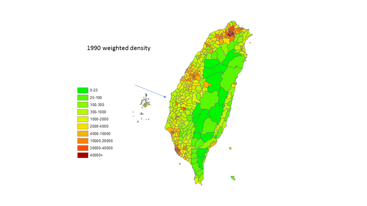
What does this look like on a map? I thought you’d never ask. Compare a regular population density map with weighted population density. The urban areas suddenly look much larger and much denser, especially in the north.

Weighted population density is always greater than population density. Theoretically, it could be equal, but in practice there is always some inflation. The question is simply how much inflation there will be. If the original area (city, town, county, country) has the same population density everywhere, then the weighted density will not be much greater than the conventional density. If there is a large amount of variance, though, the two numbers might be very different. For example, take the southeastern corner of the Taichung metro area. This is a map of population density by li in three districts: East, Dali, and Taiping. (East is upper left; Dali is lower left; Taiping is on the right.) Years ago, when I used to live in that area, I often wondered why people thought of them so differently. Taiping and Dali didn’t see any less citified than East to me. The official population densities insist that these are differences. East and Dali are cities, though hardly dense ones (8119, 7282, respectively). Taiping is suburb, perhaps maybe not even a part of the urban area (1542). On the map you can see the problem with this. Two-thirds of Taiping’s land is mountainous with fewer than 100 people/km2. The city part, however, is real city. If anything, it looks a bit more dense than neighboring East. Weighed density tells us that these two places are roughly the same. East, which has roughly the same density everywhere, is barely inflated at all (9966). Taiping is inflated significantly, to 10940. Like Taiping, Dali has quite a bit of variance in its density. Unlike Taiping, though, the sparsely populated areas only make up a small part of Dali’s overall territory. Its weighed density (18099) tells us that it is significantly more urbanized than either East or Taiping. Compared to the raw density, the weighted density for Taiping has been inflated 7.09 times; for Dali, 2.49 times; and for East, only 1.23 times.

Remember that I started this with data from 1990? Hey, let’s look at the data from 1990! Here’s a map of each town’s weighted density back then. You might notice that there is an arrow pointing to an orange town in south-central Taiwan. That town is Beigang 北港鎮. I e or less expected to see all the other dense places, but Beigang took me by surprise. If you had told me there would be one fairly dense place between northern Changhua and Chiayi City, I might have guessed Douliu 斗六市, Erlin 二林鎮, Huwei 虎尾鎮, and Xiluo 西螺鎮 before I guessed Beigang. Normal population density doesn’t indicate anything special about Beigang. The conventional population density in 1990 was only 1197, but the weighted density was 12020, an order of magnitude higher. How does that happen? Look at the picture of Beigang (1990 on left; 2016 on right). A whole heaping chunk of the population was jammed into a tiny urban area. That dense little area adds up to almost exactly one square kilometer, and in 1990 it held about 22,000 people. The rest of the town had about 27000 people in 40 square kilometers. Most city cores taper off gradually; Beigang goes from dense city straight to rural countryside with almost no transition. I confess I don’t remember much about the town except for the market right near the spectacular temple. I have no idea if there is some natural barrier that separates the city center from the rest of the town. The discovery that Beigang was a dense (if tiny) city makes me wonder about the birth of the Tangwai in Yunlin. Su Tung-chi 蘇東啟 started from Beigang in the early 1960s, and now it seems possible that he was a product of urban discontent, similar to Kao Yu-shu 高玉樹, Hsu Shih-hsien 許世賢, Huang Hsin-chieh 黃信介, Ho Chun-mu 何春木 and many of the others. (Former Yunlin county magistrate and current legislator Su Chih-fen 蘇治芬 is Su Tung-chi’s daughter. After he was arrested, her mother Su Hung Yueh-chiao 蘇洪月嬌 and elder sister Su Chih-yang 蘇治洋 were elected to the provincial assembly.)

You’ll notice that Beigang doesn’t stick out on the 2016 map. By 2016, its weighted density had plunged to only 7606 due to two trends that I’ll turn to now.

First, let’s turn away from population density momentarily to consider raw population growth. From 1990 to 2016, the overall population grew from 20.5 million to 23.4 million, or just about 15%. This map shows the ratio of 2016 to 1990 population, so anything below 1.15 is below the national average.

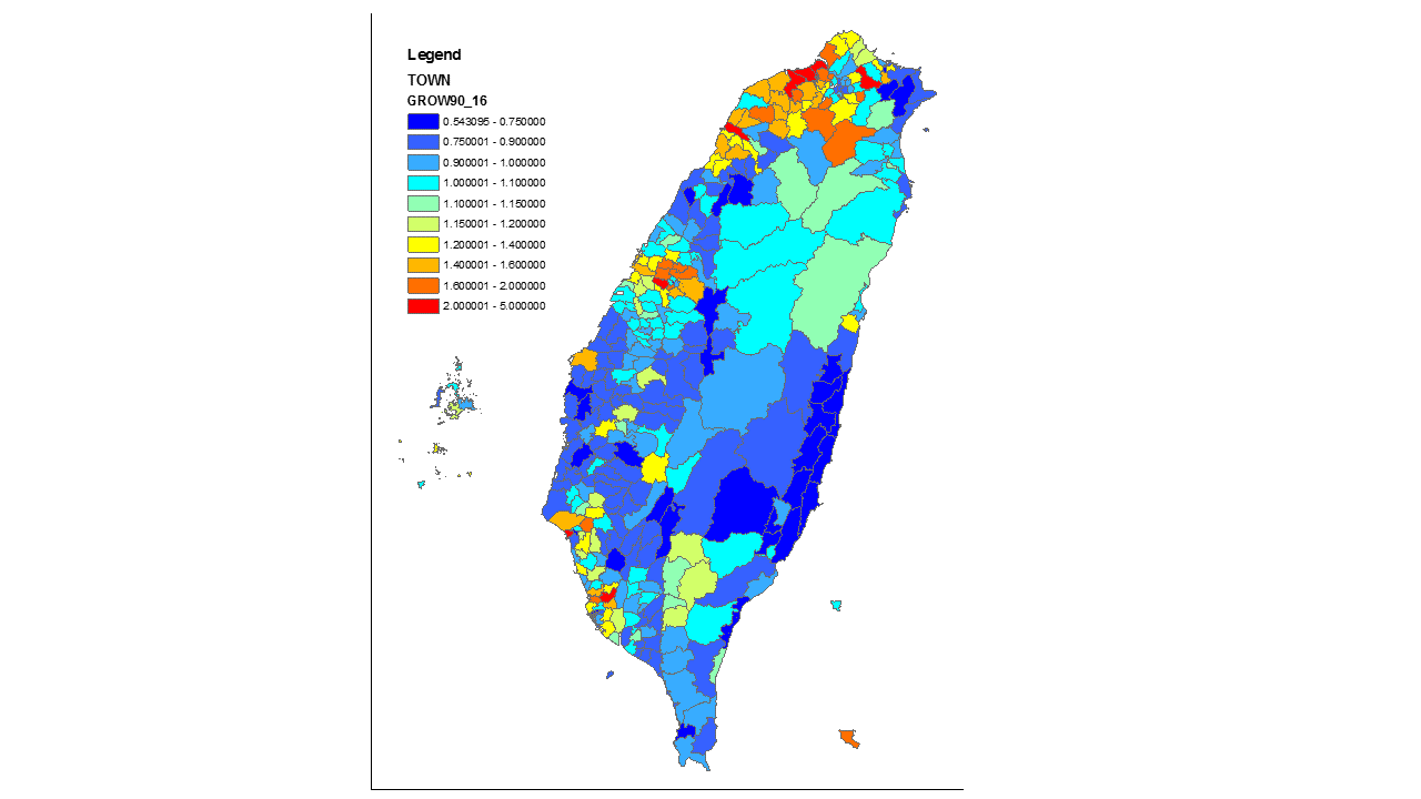
All the growing areas – the yellow, orange, and red areas – are in the north and the major urban areas. The rural areas, especially on the east coast and in southern Taiwan, are a sad, sad sea of blue and darker blue. These places have been losing population for the past 25 years, some of them at an alarming rate. There are two exceptions. Many of the majority indigenous townships are holding steady, or at least losing population more slowly than the nearby Han townships. My guess is that this reflects higher birthrates among indigenous people. The other is that single bright orange dot on the west coast, about halfway between Taichung and Tainan. That town is Mailiao 麥寮鄉, home to the huge Formosa Plastics plant. Mailiao has grown 42% while all the nearby towns have shrunk by about 20%. My guess is that an overwhelming majority of my readers have negative attitudes toward huge petrochemical facilities like the one in Mailiao. For you guys, this dot of orange in an ocean of unhappy blue is just something to keep in mind.

I said that there are two trends behind Beigang’s decline. The first is that rural areas, including Beigang, are losing population. The second trend is that city cores are also losing population. The big cities are growing, but this growth is in the ring around the old city core. I like to think of urban growth as a donut. Taichung has the cleanest example. The old city core has lost population, with the densest areas having lost the most. Central District is so tiny that it is hard to see that it is dark blue; its raw population density plunged from 39131 to 21251. East, West, and North Districts are also blue, but they are surrounded by a ring of orange and red. There is a second half ring to the west of slower growth. Then there is a light blue ring around that, and finally a dark blue ring around that one. Metro Taichung is growing, but it is doing so by spreading out rather than by piling more and more people into the city center.

Tainan and Kaohsiung are bounded by the ocean to the west, so they have half donuts rather than full donuts around them. However, the basic pattern is the same.

Northern Taiwan is more complicated. You can see donuts forming around Taipei and Keelung, but they run together a bit. To the west, there is just one huge mess of growth all the way through Taoyuan City to Hsinchu City.

This map of population growth obscures some uneven growth. Consider the difference between Xizhi汐止, just to the east of Taipei City, and Guishan 龜山, on the eastern edge of Taoyuan. Xizhi has doubled in population since 1990, but different areas have grown at different rates. In 1990 (left map) most of the population was concentrated in the old downtown area near the train station. Xizhi has grown everywhere, including in this old downtown area. However, there is basically an entirely new population center in the northwestern border, next to the Donghu area of Neihu (in Taipei City). The city has spread out, but this population center has grown so fast that it is as dense or even denser in 2016 than the old downtown area was in 1990. As a result, the weighted density has grown (from 6471 to 14817) even faster than the raw density (from 1363 to 2772).

Guishan is a different story. In 1990, the population was highly concentrated in the southwest corner, an area adjacent to Taoyuan City (now Taoyuan District). Over the past 25 years, the Taipei metro area has grown out to the edges of New Taipei City. Guishan has gotten some of the overflow. The new growth in Guishan is concentrated on the northern and eastern borders, where Guishan abuts Linkou and Taishan Districts. The new airport MRT line goes through Linkou, which in recent years has been a hot real estate market. Guishan has gotten a bit of the overflow growth from this boom. However, the newer population areas in Guishan are not as dense as the old areas. As a result, even though the overall population has grown by 60%, the weighted density is actually quite a bit lower (from 9024 to 7124). On the map of change in weighted density in northern Taiwan, Guishan is a conspicuous blue patch in a sea of orange.

This leads us to the final and perhaps most surprising result of all. Taiwan has grown by 15% over the past 25 years, and there has been heavy migration from rural areas to the cities. One might expect that this would lead to a more densely populated country. However, because the cities have spread out, with most of the growth coming in the less dense areas, weighted density insists that Taiwan is a less densely populated place today than in 1990. In 1990, the weighted density was 15457 people/km2; in 2016, that figure has fallen to 14893. By this metric, Taipei, New Taipei, Keelung, Chiayi City, Tainan, and Kaohsiung are all less dense than they used to be. The only places with significant increases are Taoyuan, Taichung, and Hsinchu County. There are more people, but the typical person lives in a less concentrated neighborhood. This finding utterly shocked me.